Have you ever played-turn based strategy games from series like Heroes of Might and Magic, Civilization, or Age of Wonders? Or maybe you would like to make a game like this yourself? 

In games of this type, movement is typically based on squares or hexes. What we usually need is to find the path to the selected point, avoiding all obstacles. It should also be the shortest path, because characters often have limited movement or action points to spend in their turn. 

This tutorial explains step by step how one of the pathfinding algorithms – A* algorithm – works using examples on squared tiles and hexes. 

A* is a complete and optimal algorithm. That means if any solution exists it will always find it and we are sure that it will always be the shortest path. So, it looks like this is what we need. 

A pathfinding issue 

Let’s look at how A* works in practice. In our example, a cat wants to reach a ball of yarn to have some fun. However, the cat is very lazy and always moves along the least involving path. 

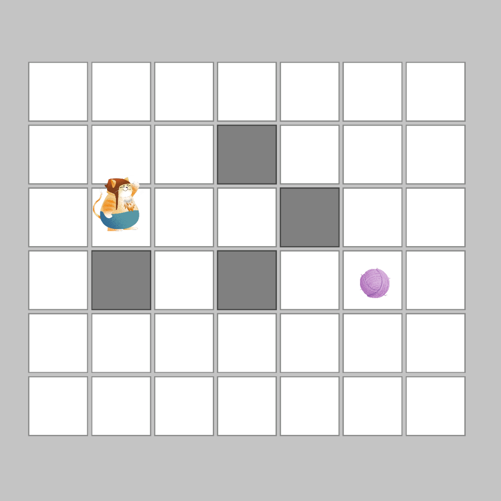
The area around the cat was split into square tiles. Some of them are occupied by obstacles, so the cat can’t get to the goal in a straight line.

Open and closed List 

Let’s see what is required for the algorithm to work. First, we’ll need two lists:

• Open list will contain all tiles that can be considered as path points.
• Closed list will contain all tiles that have already been considered. 

But how would we know in what order we should examine the given tiles? We need to somehow compute a value for each considered tile. To do this, each tile will be assessed with three parameters: F, G, and H. Let’s take a closer look at them. 

What is G? 

We start with a parameter called G. G is our current movement cost we have to spend to move from the starting point to the current considered tile. In our case we will assume that movement cost to any adjacent tile is just 1. So, by going through 5 tiles, our total movement cost will be 5. Of course, nothing stands in the way of having tiles with different costs. Moving to an area with, e.g., swamps may cost our hero more movement points.

A word about H 

H is the estimated movement cost from the current considered tile to target tile. We do not know what obstacles await us in the next steps, but we have to know whether we are getting closer to our destination or moving away, so that’s why we need to use some kind of heuristic. In our case, we use Manhattan distance, just to calculate how many tiles remain to the target point. 

For each tile, we can write its coordinates on two axes; x and y. Having the coordinates of the tiles, we can easily calculate the distance between them using the formula: 

H = |x1 – x2| + |y1 – y2| 

This is how our grid with the presented (x, y) coordinates looks:

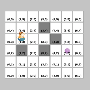
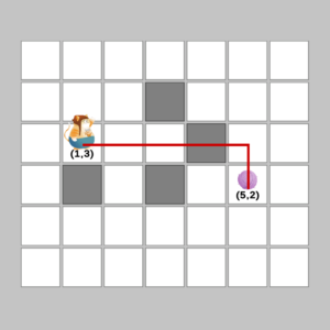
To calculate the distance from start point (1, 3) to destination point (5, 2) we substitute the values into the formula: 

H = |1 – 5| + |3 – 2| = 4 + 1 = 5

Finally F 

The simplest value. F is just the sum of G and H: 

F = G + H 

A* Algorithm 

How does the A* algorithm work? The algorithm begins by having the starting tile in its open list, then it repeats the following steps until it finds a target: 

1. Take a tile from the open list. 
2. Add this tile to the closed list. 
3. For every walkable adjacent tile of this tile:
   • If an adjacent tile is in the closed list – ignore it.
   • If an adjacent tile is not in the open list – add it to the open list. 
   • If an adjacent tile is already in the open list – check if its F parameter will be lower when we use the current path, if it is – update the adjacent tile parameters. 

At which point should we end the algorithm? Well, there are two cases. First, the algorithm will find the target tile, then we only have to determine the final path (more about that in the ‘Backtracking’ section). In the second case, we have no more elements in the open list -that means – to our misfortune – the path was not found. 

Don’t worry if you’re still a bit confused, let’s explain it with an example. 

Finding Path 

At the very beginning, before we start the main loop, we add a start point to our open list. The movement cost (G) of this tile is 0, because the cat is already on it. The estimation movement cost (H) is 5 as we calculated earlier, and the sum (F) is 0 + 5 = 5.

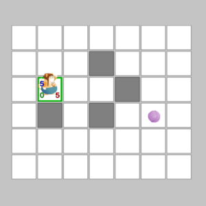
For clarity, the sum (F) is placed in the top left corner. The movement cost from the starting point to this tile (G) is in the bottom left corner, and the estimated movement cost from this tile to the destination point (H) is placed in the bottom right corner. 

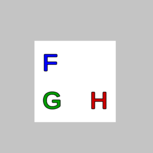
Now, we start to realize steps in the algorithm loop. We take the only element from the open list and we put it in the closed list. Then we check and calculate every walkable adjacent tile. 

Step 1

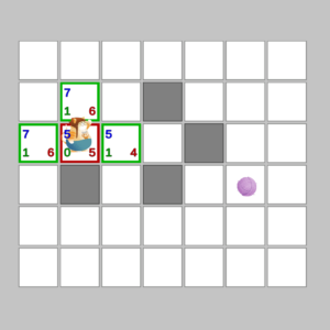
We have added three adjacent tiles to the open list (omitting non-walkable obstacle on the bottom). Note that their G value is increased by 1, we also calculate the heuristic from adjacent tiles to the destination using the aforementioned Manhattan distance. 

In the next step, we choose a tile with the lowest F value, so, in this case, it will be the tile to the right of the starting point.

Step 2

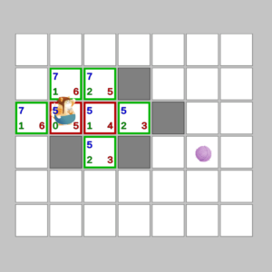
We added another three elements (omitting the element on the left, because it’s already in the closed list). At this point, we have two elements with the same lowest F, G, and H. The element we choose next depends on the implementation. The most obvious option is just taking the first available element with the lowest F from the open list. 

Step 3

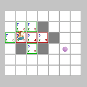
Oops. Dead end. We don’t add any new elements to the open list in this step (three adjacent tiles are obstacles and one is already in the closed list). But we still have four elements in the open list, so we continue and take the next element with the lowest F.

Step 4 

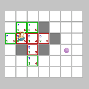
This is an interesting case. All elements in the open list have the same F value (7). What should we choose? In most cases, it’s good to continue following the current path instead of choosing a new path again and again. When we have a situation like this, we will consider elements with the lowest F, but with the highest G (as a secondary parameter), so we will continue our path. 

Step 5

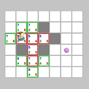
Same as above, we continue our way towards the yarn.

Step 6

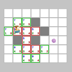
We are getting closer. 

Step 7 

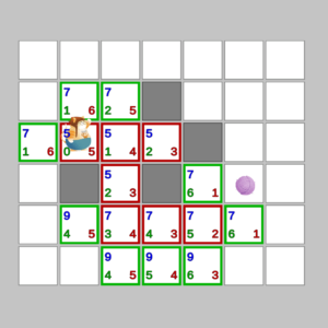
A similar situation as in step 2, two tiles with identical parameters. We just take the first tile and by chance it will be the top tile.

Step 8

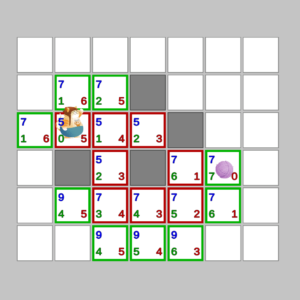
The destination tile is in the open list! In the last step, we move it to the closed list and yes, we finish the main loop. Now we need to determine the final path.

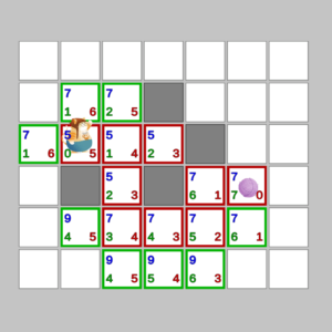
Backtracking 

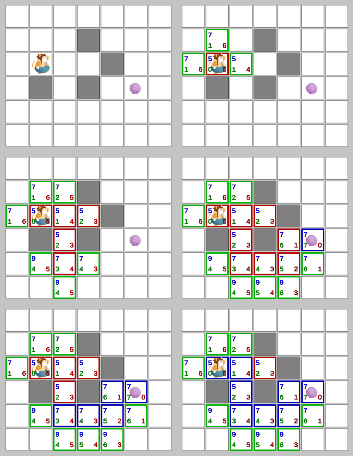
The elements in the closed list form the entire path, but it does not mean we need to use all of them. What we need to do now is called backtracking. So, to find the final path, we start with the destination tile, then we go back to the starting point. In each step, we choose an adjacent tile only if it’s in the closed list and has lower movement cost (G) than  the previous tile.

We only have to reverse the final path and that’s it. The shortest path to the yarn has been found!

Hexagon grid 

Okay, so we’ve already explained how the A * algorithm works. Now, let’s replace our tiles with a hex grid. 

A* operations on the hex grid are pretty much the same. The main change that will appear on the hex grid is how to use coordinates. We can’t just use x and y coordinates, because every second row is shifted by half-a-length. The solution is to add a third dimension and describe the hex grid by using cube coordinates. 

You can imagine it as a cube grid which we slice to create a diagonal plane.

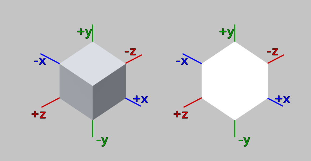
And that’s how we will represent coordinates x, y, and z.

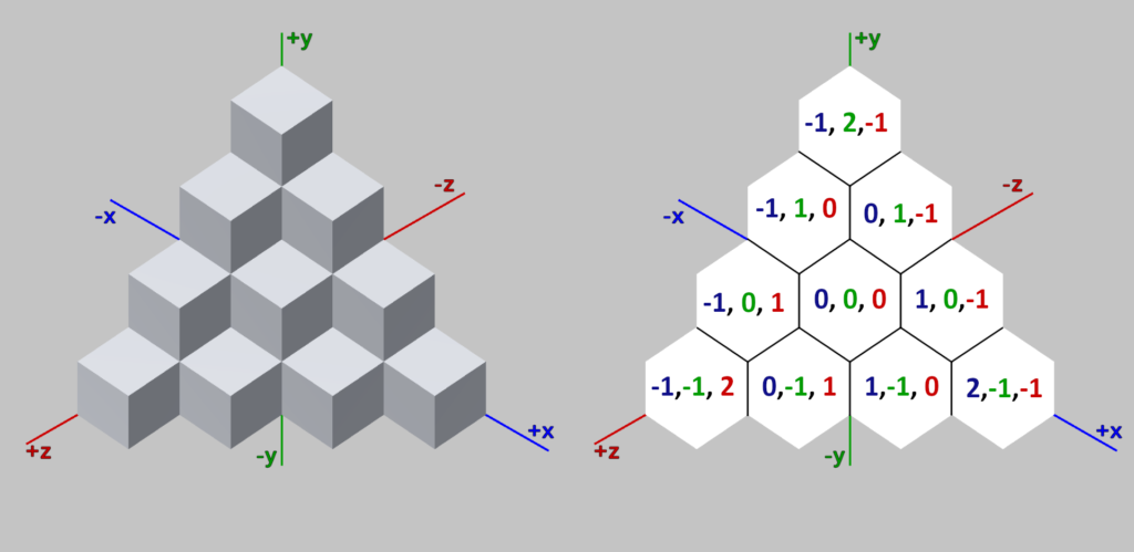
It comes down to the fact that: 

• the value on the x axis will be increased whenever we move to the right or bottom right hex and decreased when we move to the left or upper left hex 
• the value on the y axis will be increased when we move to the upper left or upper right hex and decreased if choosing the bottom left or bottom right hex
• the value on the z will be increased when we move to the left or bottom left hex and decreased for the upper right or right hex
  

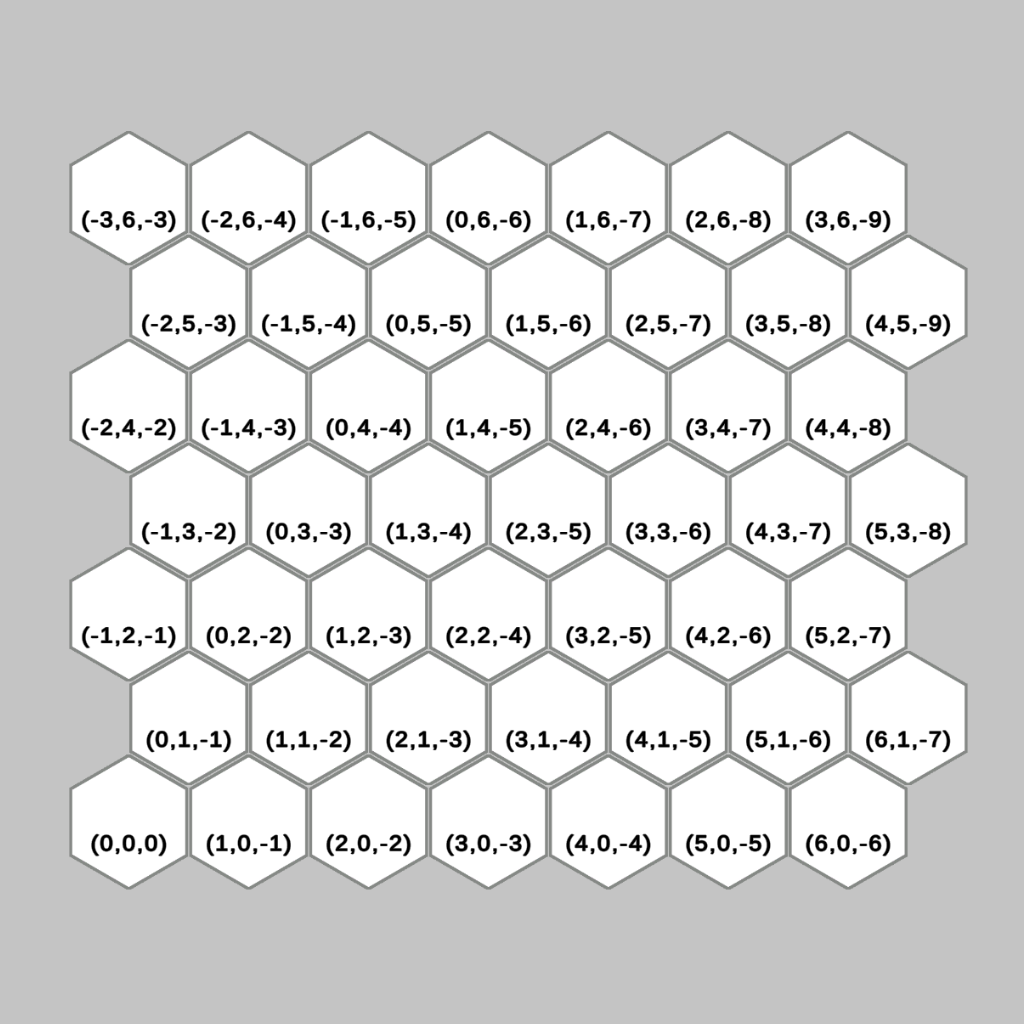
This is what our hexagon grid with saved coordinates looks like. Note one thing; the sum of all three axes is always equal to zero, x + y + z = 0. 

In this case, the formula to get the distance between any two hexes has the form: H = Max(|x1 – x2|, |y1 – y2|, |z1 – z2|) 

We calculate the absolute value of subtraction of each axis and then we take the highest value. 

Take a look at a similar example, but now let’s check how the algorithm behaves on a hexagonal grid.

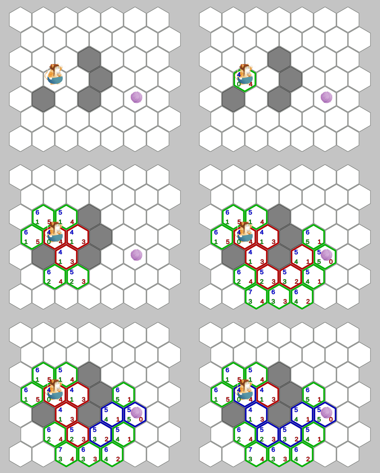
Implementation 

Now, it’s time for a simple example implementation in C#. Tile class consists of:

• F, G, and H parameters (F is just the sum of G and H so, it will be only the returning value), 
• position to calculate the distance, 
• references to its adjacent tiles, 
• info if the tile is an obstacle (if it is, it means that tile is not walkable).

Remember that the last three variables should be set up before we run the algorithm. 

Listing 1 – Click to check out! 

The FindPath method in the AStarPathfinding class requires start and end tiles. It returns a list with path points or an empty list if a path has not been found. For better readability, computing the H value was moved to a separate method. 

Listing 2 – Click to check out! 

Summary 

Hey, I hope this article helped you learn the basics of A* pathfinding and now your heroes will never get lost when exploring dangerous dungeons or when traveling through mystic lands, and they will always find the shortest path home or to the couch 🙂 

It’s worth pointing out that the A* algorithm works well not only in games that use squares or hexes. Identical solutions are also used in other games. The area, although appearing to be continuous, is actually split into a grid with a limited number of points. It’s all done to reduce the number of computations.